


 @Boston Celtics #NBA #Basketball #Celtics #JaysonTatu…


 #NBA #basketball #NBAXmas #Jalen…


 #McLaren #F1 #Gingerbread #CapCu…


 #rugby #haka


 CMA Members get access to my “AXEL TECHNIQ…


Abstract The Fitness-Fatigue Model (FFM) is a widely used model for predicting sport performance. Its key advantage lies in its ability to forecast athletes’ performance based solely on a training program, which can be preliminarily designed by their coach. Introduction Article MATH Google Scholar Article Google Scholar Pfeiffer, M. Modeling the relationship between training and […]

Abstract
Introduction
MATH
Google Scholar
Article
Google Scholar
Pfeiffer, M. Modeling the relationship between training and performance-a comparison of two antagonistic concepts. Int. J. Comput. Sci. Sport. 7 (2), 13–32. (2008)Article
Google Scholar
Article
PubMed
PubMed Central
Google Scholar
Material & methods
Data description
The authors declare no competing interests.
The 2019 dataset
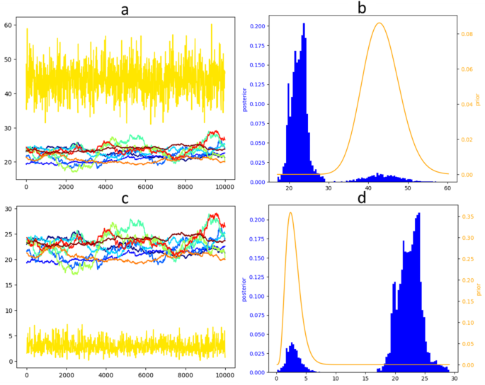
Fifteen (15) national elite Short-track speed skaters voluntary participated to a previous study18. One of the skaters was injured and removed from the study, leaving 14 athletes in. Athletes had the same coach for both datasets. Out of these 14 athletes, 2 were also represented in the 2019 data set.Bayesian modelling is a statistical paradigm that allows for combining information from observed data (the likelihood) with information from background knowledge (the prior). It also enables solving models with Monte-Carlo Markov Chains (MCMC), an approach that unveils the whole distribution of the resulting, concordant posterior estimations. On one hand, the inclusion of a prior knowledge makes a special sense in the context of a deterministic model, from which the components have a biological meaning. On the other hand, unveiling the posterior distribution is a powerful tool for the diagnosis of statistical issues such as ill-conditioning or an overall lack of information15. Tackling FFMs from a Bayesian perspective has not been done until recently16. Peng et al. identified a gain in the plausibility of the parameter estimates as compared to the frequentist counterpart (i.e. non-Bayesian, based on pure likelihood). However, the predictive ability of the FFM fitted in a Bayesian framework was not investigated by these authors16.On the other hand, the chains that did not converge exhibited a strong autocorrelation within chains for all parameters and inconsistency between chains for most parameters. In the unconverging chains, τG and τH displayed a mirror behaviour: they took a close value for a given chain at a given iteration (Fig. 4a and c, and Appendix C). The mirror posture was also observed for kG and kH that were almost identical for a given non-converged chain at a given iteration (Fig. 5, and Appendix B). Note that on Fig. 5 (and Appendix C), the sample dispersion for kG and kH for the converged chain(s) is too small to be noticeable at the given scale, and only one chain converged for this athlete.
The 2016 dataset
Using a Fitness-Only Model (FOM), we showed that the optimal value for the time exponent was not estimable from the likelihood. The Fig. 1 (c-d) exemplified this pattern: using a flat prior for the time exponent in the FOM led to estimates with no physiological sense at all. Adding biologically meaningful information to the fitness dynamic, by fixing its time exponent or by means of a bayesian prior, led to the model with the best predictive ability in cross-validation. Adding a fatigue component implies two challenges: the estimation of the fatigue time exponent itself and dealing with an antagonism between the fitness and the fatigue components during the estimation process. The diagnosis of the Markov chains used to fit the FFM in a Bayesian framework illustrated how this antagonism prevented the model from converging. Noteworthily, maxima of likelihood were easily identifiable for the fatigue time exponent when the fitness time exponent had been fixed, but never when both parameters were simultaneously estimated. Consequently, augmenting the model complexity with supplementary state variables (i.e. fatigue) does not ensure enhanced model performance, as parsimony appears to prevail in time-invariant FFMs23.Ludwig, M., Asteroth, A., Rasche, C. & Pfeiffer, M. Including the past: performance modeling using a Preload Concept by means of the fitness-fatigue model. Int. J. Comput. Sci. Sport. 18 (1), 115–134. https://doi.org/10.2478/ijcss-2019-0007 (2019).In the previous section, we observed that providing information for τG was beneficial to the predictive ability of the model. This questions the appropriate value to which τG should be informed. We addressed this question by the mean of a grid search. The grid ranged from one day to 100 days with a step of 1 day for the fitness half-life. The time exponent parameter τG was computed according to each fitness half-life, fixed to this value, and all other parameters (a0, kG, σ²) were estimated. The fitness (Fig. 3a) and the predictive ability (Fig. 3b) of the model were then assessed.
Models
Article
PubMed
MATH
Google Scholar
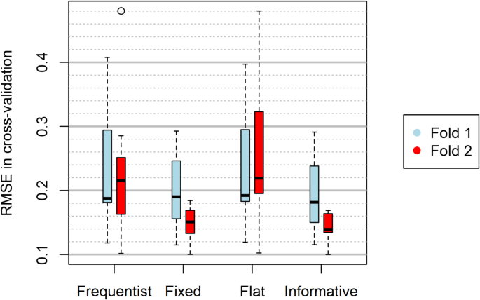
RMSE in cross-validation depending on the way the fitness-only model was fitted. The boxplot corresponds to the 7 athletes for each fold of the cross-validation. “Frequentist”: all parameters, including τG, were directly estimated by minimization of the RMSE in the training set. “Fixed”: is identical to “Frequentist” with the exception that τG was fixed to 43.28 (corresponding to a half-life of 30 days). “Flat” and “Informative” correspond to bayesian fitting with a gamma distribution for τG. “Flat”: the prior for τG was Γ(a = 1, b = 0.5). “Informative”: the prior for τG was Γ(a = 2 × 43.28, b = 2).
You can also search for this author in
PubMed Google ScholarYou can also search for this author in
PubMed Google Scholar
Racine, J. Consistent cross-validatory model-selection for dependent data: hv-block cross-validation. J. Econ. 99 (1), 39–61 (2000).
Model fitting
Prior knowledge on the time exponents
A frequentist framework where all parameters are estimated;
Matabuena, M. & Rodríguez-López, R. An Improved Version of the classical Banister Model to Predict Changes in Physical Condition. Bull. Math. Biol. 81 (6), 1867–1884. https://doi.org/10.1007/s11538-019-00588-y (2019).
Frequentist model fitting
Seenovate, Paris, 75009, FranceDMeM, INRAe, Univ Montpellier, Montpellier, 34000, France
DOI: https://doi.org/10.1038/s41598-025-88153-7
Bayesian model fitting
Non-convergent chains for τG and τH did not converge for the other parameters neither;Busso, T. Variable dose-response relationship between exercise training and performance. Med. Sci. Sports Exerc. 35 (7), 1188–1195 (2003).Stan Development Team. – Stan Modeling Language Users Guide and Reference Manual. Available at: https://mc-stan.org (2023).
Cross-validation
The predictive ability of the models was assessed by the mean of cross-validation. Since we deal with time series, the data were time-ordered and split accordingly in subsets in respect of hidden-value block cross-validation with an incremental window12,22. We used minimal values of 35 days and 15 days for training and test sets, respectively. Due to potential dependencies between training and test data, a 5-day gap between each training and test subsets was considered to ensure unbiased model predictions. This parameterization yielded 2 folds for the 2019 dataset and 3 folds for the 2016 dataset as described in Table 2.
Using a Bayesian framework, we found that some parameters could not be estimated solely from the available data. However, the model demonstrated a strong capacity to incorporate prior information. The formulation incorporating prior knowledge about fitness dynamics outperformed all others in this study.
Results
Estimation of the fitness time exponents
Informativeness for the fitness time exponent
- We used root mean square error (RMSE) between predicted and observed performance to quantify the predictive ability of the models. RMSE of the training data, i.e. the residual deviation of the model σ, was also employed to measure the goodness of fit of a model to its training data.
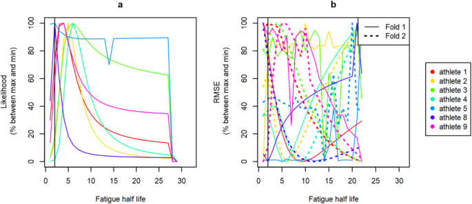
- Maxima of likelihood emerged for τH in the investigated range and for all athletes. These maxima were specific to each athlete and comprised between fatigue half-life = 2 days (⇔ τH = 2.89) to fatigue half-life = 6 days (⇔ τH = 8.66) (Fig. 6a). These maxima of likelihood were not associated with better predictive abilities, excepted for fold 1 of athlete 8 and fold 1 of athlete 4 (Fig. 6b).
- Following a 15-minutes standardised warm-up, participants performed weekly flying starts for a one-lap maximal run. Four photocells were settled for recording skating times. The dependent variable further modelled was the individual maximal acceleration (from speed derivation); hence a higher performance value was sought. On-ice and off-ice training sessions were used as the explanatory variables, as described by Méline et al.18 and consistently with the 2019 dataset.
- This is referred to as the fitness-only model (FOM) in this study.
We considered the Banister’s fitness-fatigue model (FFM) from a stochastic perspective, in which the predicted performance of athlete s at time t: (:y_sleft(tright)), was considered as the expectation from a gaussian distribution:Initiating the model state variables with relevant values has a potential implication in the inference26. Null state variables come with the assumption of modelling performances of untrained athletes, which is usually not realistic. Consequently, we investigated simulations of previous training session (up to 2 years priors to the observed datasets) to start from non-null fitness and fatigue states. However, it did not lead to a reliable improvement of the predictive ability of the model, neither for the FOM, neither for the FFM model (data not shown).
Grid search for an optimal fitness time exponent
Article
PubMed
MATH
Google Scholar
Sorry, a shareable link is not currently available for this article.
Estimation of the fatigue time exponents
Informativeness for the fatigue time exponent
Non-convergent chains exhibited a mirroring pattern with nearly identical τG and τH, and kG and kH for a given chain at a given iteration.Thibaut MélinePeng, K., Brodie, R. T., Swartz, T. B. & Clarke, D. C. Bayesian inference of the impulse-response model of athlete training and performance. International Journal of Performance Analysis in Sport, 24(1), 74–89. https://doi.org/10.1080/24748668.2023.2268480 (2023).We compared two strategies for the time exponent estimations. On the one hand, we used non-informative priors (:tau:_GsimvarGamma:(a=1,:b=0.5)) which is equivalent to a (:upchi:^2) distribution with 2 degrees of freedom; same for (:tau:_{H}). On the other hand, we fitted the models with informative priors for the time exponents: (:tau:_GsimvarGamma:(a=2*43.28,:b=2)) and (:tau:_{H}simvarGamma:(a=2*2.89,:b=2)). The average of a gamma distribution defined by its shape (a) and rate (b) is a/b, hence these priors are consistent with the background knowledge target as developed in 2.3.1. We emphasize that these targets have been designed without information from the data. The rate parameter b = 2 was set high but not extreme.
Hellard, P., Avalos, M., Lacoste, L., Barale, F., Chatard, J. C. & Millet, G. P. Assessing the limitations of the Banister model in monitoring training. J. Sports Sci. 24 (5), 509–520. https://doi.org/10.1080/02640410500244697 (2006).
Grid search for an optimal fatigue time exponent
Calvert, T. W., Banister, E. W., Savage, M. V. & Bach, T. A systems model of the effects of training on physical performance. IEEE Trans. Syst. Man. Cybern Syst. 2, 94–102 (1976).Alexandre Marchal, Othmène Benazieb, Yisakor Weldegebriel & Frank Imbach
Performance of the fitness-fatigue model
Marchal, A., Benazieb, O., Weldegebriel, Y. et al. Statistical flaws of the fitness-fatigue sports performance prediction model.
Sci Rep 15, 3706 (2025). https://doi.org/10.1038/s41598-025-88153-7For two athletes (athletes 3 and 5, see Appendix B), kH exhibited instability that was expressed in the converged chains: it wandered to extreme values before coming back to the maximal density area of the chain. These expeditions caused local autocorrelation for kH and were locally associated with close-to-0 samples for τH.
Confirmation on a new independent dataset
Informativeness for the fatigue time exponent
Accepted:
- The performance data were collected each week and consisted in the time to perform a 166.68 m race after a standardised warm-up; hence a lower performance value was sought. Timing gate systems (Brower timing system, USA) were used to record valid individual time trial performance17. On-ice and off-ice training loads were used as the explanatory variable as described in the Appendix 1 from Imbach, Perrey, et al.12.
- Conceptualisation, A.M., F.I.; methodology and investigation, A.M., Y.W., O.B., F.I.; data curation, T.M., Y.W.; recruitment, T.M.; resource development, A.M., Y.W., O.B.; formal analysis, A.M.; writing original draft preparation, A.M., F.I.; writing-review and editing, A.M., Y.W., O.B., F.I.; supervision, F.I.; project administration, F.I. All authors have read and agreed to the published version of the manuscript.
- A frequentist framework with the fitness time exponent τG being fixed to 43.28 (see Sect. 2.3.1 for details);
- A Bayesian framework with an informative prior for τG.
Article
CAS
PubMed
Google Scholar
Vermeire, K., Ghijs, M., Bourgois, J. G. & Boone, J. The fitness–fatigue model: what’s in the numbers? Int. J. Sports Physiol. Perform. 17 (5), 810–813. https://doi.org/10.1123/ijspp.2021-0494 (2022).
Performance of the fitness-fatigue model
The identifiability of τG and τH was investigated in a Bayesian framework with informative priors (see Fig. 4 for a representative athlete and Appendix B for all athletes involved in the 2019 dataset).
Discussion
Practical considerations
- of variance (:sigma:_s^2) and expectation (:widehaty_sleft(tright)) a function of the daily training doses or workloads (:w_sleft(iright))1:
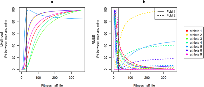
- Quality of the fitness-fatigue model fitted with fixed values for the time exponent τH. The time exponent is computed from the resulting half-life for fatigue, provided as the x-axis and varying from 1 to 29 (a) and 1 to 22 (b). Plot (a) shows the quality of fit in the training processus, assessed using the likelihood. Plot (b) shows the predictive ability assessed as the RMSE for each fold (fold 1: plain line and fold 2: hashed line). Each athlete is represented with a different color detailed in the legend. Likelihood and RMSE in prediction are returned as percentage of the difference between their maximum value and their minimum value on the y-axis. The vertical black line corresponds to x = 2 days, i.e. the half-life we informed elsewhere in this paper.
- kH was very instable in converged chains, frequently wandering at extreme values;
- Busso, T. & Chalencon, S. Validity and accuracy of impulse-response models for modeling and Predicting Training effects on performance of swimmers. Med. Sci. Sports Exerc. 55 (7), 1274–1285. https://doi.org/10.1249/MSS.0000000000003139 (2023).
Data availability
References
- Not all issues with the FFM transposed to the FOM. The Markov chains of the FOM converged when provided some information. A few combinations of athletes and folds showed an optimal value for τG in terms of predictive ability, that was close to our prior conception of a half-life of 30 days for a gain in fitness (Fig. 3b). This suggests that in these few situations, the fitness time component may have captured a biological phenomenon with which our prior idea of the magnitude was consistent. The data likely misses the information for this result to be reproducible to each athlete and to each fold since we worked with relatively short time series (less than 3 months including a 2-week summer break). Nevertheless, the FOM presents strong assets: (i) it is not affected by the structural ill-conditioning due to the antagonism between fitness and fatigue components, as discussed so far; (ii) it still allows for tackling the asynchronicity between trainings and performance, which is fundamental in the sports performance applications; (iii) it allows pure prediction on the basis of a training program; (iv) the fitness value may be directly interpreted by athletes, coaches and sport professionals as an actual performance potential at a given time for a given athlete. The points (iii) and (iv) are obviously conditional on the predictive ability of the model that may vary from one situation to the other.
- A total of 948 training and 755 performance observations were collected, distributed as 67.7 ± 5.6 training observations and 53.9 ± 5.4 performances per athlete. The period of study included 13 weeks from July to October. During this period, the skaters sustained a mean weekly training volume of 25 ± 5 h.Appendix C displays FOM and FFM outputs from the independent 2016 dataset. Note that the 2016 and 2019 datasets share 2 common athletes, which make them somewhat related. However, they are considered independent due to the time gap between them and, more generally, because the performance criteria differ. Both models were fitted in a Bayesian framework with informative priors for τG and τH. Among the 14 athletes included in the 2016 dataset, 6 did not show any convergent Markov chains for the FFM (athletes F5, H2, H5, H6, H11 and H13, see Appendix C). The other height athletes had between 1 and 3 converged chains out of 10. The conclusions are identical to the ones drawn from the 2019 data (Figs. 5 and 6, Appendix B):
- Received:
- One to four Markov chains converged out of 10 for any athlete, and convergence always occurred within the peak density of the prior for both τG and τH (Fig. 4a, b, c and d, respectively; see Appendix B for all athletes). The convergence of τG and τH was always associated with the convergence for all other parameters (a0, kG, kH, σ).For all athlete, bunching the 10 chains (i.e. chains that converged in the peak density of the prior and chains that did not converge at all) led to poor model properties (Appendix B). These results were even worse when using flat priors or a frequentist framework for estimating τG and τH (results not shown). Since non-convergence of Markov chains discredit the models, we fixed τG and τH for the rest of this investigation.
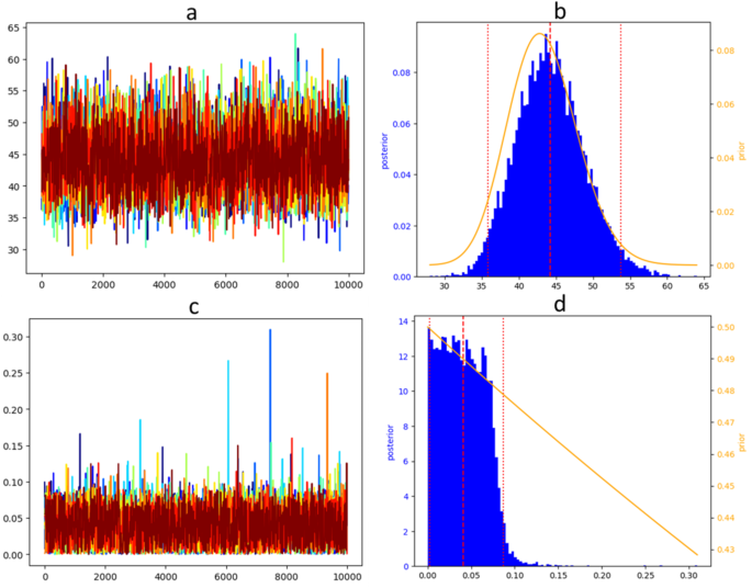
- Morton, R. H., Fitz-Clarke, J. R. & Banister, E. W. Modeling human performance in running. J. Appl. Physiol. 69 (3), 1171–1177 (1990).The prior had a strong influence on the posterior for τG, suggesting that it carried more information than the data itself for the estimation of this parameter (see Fig. 1a for a representative athlete, Appendix B for all other athletes from the 2019 dataset). Accordingly, following an informative prior, the posterior distribution embraced almost perfectly the prior distribution (Fig. 1b, Appendix B).
- Below is the link to the electronic supplementary material.This study demonstrates that the FFM has significant statistical limitations. Further research is necessary to develop a more reliable model formulation, particularly to address the challenges of performance prediction when designing training programs.
- Modelling the effects of training on performance has been extensively studied over the last five decades. A historical approach has been driving research with the statement of a dose response relationship between exercise and performance, through fitness and fatigue states variables1,2,3,4. The so-called Fitness-Fatigue Model (FFM) is deterministic and based on a schematisation of the biological processes underpinning physical exercise5. In its simple form, it assumes that a training dose induces two antagonistic responses, the fitness representing incremental, long-lasting positive adaptations of the body and its physiological processes; and the fatigue standing as intense, short-lasting inhibition of the performance potential. From a mathematical perspective, fitness and fatigue states variables are derived from first order differential equations in which the training dose is expressed as a discrete function and convolved with an exponential transfer function. Then, the predicted performance is given by the difference between states variables that serves as a proxy of global physiological adaptations to training doses, responsible for athletic performance5,6. Considering the explicit and algebraic formulation of the model, FFMs provide the explicit solution that would maximize the performance without performing simulations of training doses4.Correspondence to
Frank Imbach. - Lambert, E. V., Gibson, A. S. C. & Noakes, T. D. Complex systems model of fatigue: integrative homoeostatic control of peripheral physiological systems during exercise in humans. Br. J. Sports Med. 39 (1), 52–62 (2005).Quality of the fitness model fitted with fixed values for the time exponent τG. The time exponent is computed from the resulting half-life for fitness, provided as the x-axis and varying from 1 to 365. Plot (a) shows the quality of fit in the training processus, assessed using the likelihood. Plot (b) shows the predictive ability assessed as the RMSE for each fold (fold 1: plain line and fold 2: hashed line). Each athlete is represented with a different color detailed in the legend. Likelihood and RMSE in prediction are returned as percentage of the difference between their maximum value and their minimum value on the y-axis. The vertical black line at x = 30 days correspond to the value that was used to fix τG throughout this paper or to inform it in the bayesian prior.
- Fixing τG or providing its information in the prior yielded to close parameter estimates, hence close predictive performances (Fig. 2). On the other hand, using a Bayesian framework with non-informative prior for τG or estimating τG in a frequentist framework resulted in poorer predictive performances (Fig. 2). The differences between approaches using information (with Bayesian informative priors or fixed parameters) versus estimating τG only from the data (with Bayesian genuine priors or frequentist estimation of the parameters) were close to significance, as seen in Table 3.Anyone you share the following link with will be able to read this content:
- The data collection spread over 10 weeks, from June to September. The period of study was interrupted by a two-week summer break, during which athletes fully rested. Skaters sustained a mean weekly training volume of 16.6 ± 2.5 h during this period. A total of 375 training and 248 performance observations were collected, distributed as 53.6 ± 1.6 training observations and 35.4 ± 2.2 performances per athlete.Models were also fitted in a bayesian framework. We used proper, mildly informative priors for (:a_{0}sim:N(0,{5}^2)) ; (:k_G=-left|Xright|) (for the 2019 dataset) (or (:k_G=+left|Xright|) for the 2016 dataset), with (:Xsim:N(0,{5}^2)); idem for (:k_{H}) ; and a flatter prior for (:{upsigma:}:=:left|Xright|) with (:Xsim:N(0,{25}^2)). Half-normal distribution is part of the half-Student distribution family, which are generally advised for variance parameters priors20.
- Mujika, I., Busso, T., Lacoste, L., Barale, F., Geyssant, A. & Chatard, J. C. Modeled responses to training and taper in competitive swimmers. Med Sci Sports Exerc., 28 (2), 251–258. (1996).Optimizing athletic training programs with the support of predictive models is an active research topic, fuelled by a consistent data collection. The Fitness-Fatigue Model (FFM) is a pioneer for modelling responses to training on performance based on training load exclusively. It has been subject to several extensions and its methodology has been questioned. In this article, we leveraged a Bayesian framework involving biologically meaningful priors to diagnose the fit and predictive ability of the FFM. We used cross-validation to draw a clear distinction between goodness-of-fit and predictive ability. The FFM showed major statistical flaws. On the one hand, the model was ill-conditioned, and we illustrated the poor identifiability of fitness and fatigue parameters using Markov chains in the Bayesian framework. On the other hand, the model exhibited an overfitting pattern, as adding the fatigue-related parameters did not significantly improve the model’s predictive ability (p-value > 0.40). We confirmed these results with 2 independent datasets. Both results question the relevance of the fatigue part of the model formulation, hence the biological relevance of the fatigue component of the FFM. Modelling sport performance through biologically meaningful and interpretable models remains a statistical challenge.
- Turner, J. D., Mazzoleni, M. J., Little, J. A., Sequeira, D. & Mann, B. P. A nonlinear model for the characterization and optimization of athletic training and performance. Biomed. Hum. Kinet. 9 (1), 82–93 (2017).Springer Nature remains neutral with regard to jurisdictional claims in published maps and institutional affiliations.
- Download referencesGelman, A. Prior distributions for variance parameters in hierarchical models. Bayesian Analysis, 1 (3), 515–533. (2006).
- Kolossa, D., Bin Azhar, M. A., Rasche, C., Endler, S., Hanakam, F., Ferrauti, A. & Pfeiffer, M. Performance estimation using the fitness-fatigue model with kalman filter feedback. Int. J. Comput. Sci. Sport. 16 (2), 117–129 (2017).On the other hand, FOM (Appendix C) showed convergence for all 10 chains and for all athletes. Convergence happened for τG within its densest prior segment, or near to it. The greatest difference between the prior and the posterior was observed for athlete H10 (see Appendix C), suggesting the expression of a slight information from the data likelihood for this athlete. All other parameters (a0, kG, σ) converged for all athletes and Markov chains.
- The time exponents (τG and τH) only converged in the peak density of the prior;Kataoka, R., Vasenina, E., Hammert, W. B., Ibrahim, A. H., Dankel, S. J. & Buckner, S. L. Is there evidence for the suggestion that fatigue accumulates following Resistance Exercise? Sports Med. 52 (1), 25–36. https://doi.org/10.1007/s40279-021-01572-0 (2022).
- Though the fatigue component captured an appreciable amount of variance in the training data once the fatigue time exponent had been fixed, it did not contribute to the predictive ability of the model in cross-validation. Overfitting is characterized by an increased model complexity leading to a gain in the goodness of fit that does not translate into a better predictive ability. From this definition, overfitting issues can only be tackled with a test dataset unconsidered for model training. However, the FFM and derivative models are scarcely challenged in cross-validated studies12,26,27. For this reason, we partially agree with Peng et al.16 who conclude that a Bayesian approach overcomes the main challenges of a FFM. If adding information in the prior indeed helped the parameters estimation process in some cases, it has not been shown to make the fatigue component relevant with regards to the predictive ability, neither in our study nor anywhere in the literature as far as we are aware of. Models are meant to represent the real world, the lack of statistical relevance of a component questions its biological relevance. Fundamentally, it is not trivial that the fatigue as modelled in the FFM really mimics a biological phenomenon, since humans are driven by sophisticated physiological processes in interaction28,29.
- One of the main interests of the FFM is its biological interpretability. Exponential decays can be interpreted from their half-life (i.e. the amount of time needed for half the effect of an input to vanish). The time exponent value τ leading to a half-life h is:Adding the fatigue component provided to the model the ability to capture the short-lasting variations, notably the summer break effect over the modelled performance (Appendix A). Indeed, during this 2-week break, the FOM predicted a loss of performance whereas the FFM predicted a gain of performance, which turned out to be more accurate. The benefit of including a fatigue component in the model led to a reduction of 0.017 in the training set RMSE (Cohen’s d = 0.585, one-sided Student mean comparison of paired data: p-value < 0.001).
- Article
CAS
PubMed
PubMed Central
MATH
Google Scholar
Unfortunately, this better goodness of fit did not translate into a better predictive ability. The predictive ability is slightly, though not significantly, decreased when providing a fatigue component with an addition of 0.001 to the RMSE (Cohen’s d = 0.022, p-value = 0.57). - To conclude, the FFM presents major dysfunctions that prevents its use for predictive purposes. These results are consistent with the conclusions that other authors have already reached and published. One may be tempted to use FFM to support the design of athletic training programs; these conclusions warn us against this practice. Adding prior information, for instance with a Bayesian approach, seems beneficial to the FOM. This simple model may be the starting point for further improvement, that considers other sources of information and/or an alternative transfer function from training to short-term effects on sport performance.Article
CAS
PubMed
PubMed Central
Google Scholar - Alternatively, we fixed τG and τH (see Sect. 2.3.1) before estimating the other parameters, hence reducing the system to a linear model.
- Fédération Française des Sports de Glace, Paris, France
- No optimum was found for the likelihood in the investigated interval for 6 out of the 7 athletes. Besides, the higher half-life for τG led to a higher likelihood for these 6 athletes. Only athlete 5 reported an optimum, with a maximum of likelihood given for a fitness half-life = 43 ((Leftrightarrow) τG = 62.04, see Fig. 3a). The performance in cross-validation were even more idiosyncratic, and no clear trend could be drawn. For 4 combinations of athlete and fold, an optimum appeared clearly close to the half-life suggested for τG or used in the Bayesian prior (fitness half-life = 30 (Leftrightarrow)τG = 43.28). An optimum also emerged for athlete 2 – fold 2, but with a lower value (fitness half-life = 16 (Leftrightarrow)τG = 23.08). For the 9 other combinations of athletes and folds (i.e. 64.3% of the combinations), no optimal value was found over the studied interval (see Fig. 3b).The gain in performance when adding a fatigue component using the 2016 dataset yielded to the same results than using the 2019 dataset. Indeed, the goodness of fit to the training data was slightly but significantly increased, with a reduction of 2.8 × 10− 4 in RMSE (Cohen’s d = 0.056, p-value < 0.01, one-sided Student mean comparison of paired data). Again, this gain in goodness of fit to the training data did not translate into a significant gain in predictive ability. The RMSE in cross-validation was reduced by 8.8 × 10− 5, this difference was not-significant (Cohen’s d = 0.006, p-value = 0.41).
Article
PubMed
MATH
Google Scholar
PubMed
Google Scholar
Markov chains of τG (a, b) and τH (c, d) estimated from the model with fitness and fatigue for athlete 1, using informative priors for τG ~ Γ(a = 2 × 43.28, b = 2) and τH ~ Γ(a = 2 × 2.89, b = 2). Plots a and c show the raw Markov chains, each color represents one of 10 chains, the x-axis is the iteration number and the y-axis are the τG (a) and τH (c) values. Plot (b) (respectively (d)) represent the compilation of the 10 chains represented in (a) (respectively (c)) in a blue histogram whose legend is on the left; and the prior is represented in yellow as a density function whose legend is on the right.
PubMed
MATH
Google Scholar
You can also search for this author in
PubMed Google Scholar
The fatigue component in the FFM is considered as antagonistic to the fitness component. To address this issue, alternative formulations of fatigue or new metrics with greater physiological relevance should be explored.
Acknowledgements
PubMed Google Scholar
Author information
Authors and Affiliations
Contributions
For the sake of robustness of analyses, we modelled the performance of world-class short-track speed skaters over two distinct datasets, collected in 2019 and 2016 respectively. For both datasets, participants were fully informed about data collection and written consent was obtained from them. Also, the study was performed in agreement with the standards set by the declaration of Helsinki (2013) involving human subjects. The protocol was reviewed and approved by the local research Ethics Committee (EuroMov, University of Montpellier, France). The present retrospective study relied on the collected data without causing any changes in the training programming of athletes.
Corresponding author
In the above equation, a0 denotes the intercept, kG and kH represent the linear coefficients for fitness and fatigue, respectively, and τG and τH the time exponents for fitness and fatigue, respectively. All these parameters are written with an s subscript that denotes the athlete identity, as the parameters are estimated at the individual level.
Ethics declarations
Competing interests
Additional information
Publisher’s note
Electronic supplementary material
The frequentist model fitting refers to the estimation of θ by minimizing the standard deviation σ, which is equivalent to maximizing the likelihood under Gaussian dispersion assumption (Eq. 1). The minimization was performed using the Powell algorithm from the scipy library19.
Rights and permissions
Article
MathSciNet
PubMed
MATH
Google Scholar
About this article

Cite this article
Banister, E. W. & Hamilton, C. L. Variations in iron status with fatigue modelled from training in female distance runners. Eur. J. Appl. Physiol. Occup. Physiol. 54 (1), 16–23 (1985).Article
PubMed
Google Scholar
- Bayesian fitting was performed using Markov Chain Monte Carlo (MCMC), with 10 independent Markov chains for each model fitting. Independent Markov chains were initiated from random initial values uniformly sampled within the intervals described in Sect. 2.3.2. Each chain had 4 × 10⁴ iterations warm-up, 1 × 10⁴ iterations sampling, and a 10-iteration thinning so they ended up 103 iterations long. Computation were performed using the Python implementation of Stan21.
- Philippe, A. G., Borrani, F., Sanchez, A. M., Py, G. & Candau, R. Modelling performance and skeletal muscle adaptations with exponential growth functions during resistance training. J. Sports Sci. 37 (3), 254–261 (2019).
- Download citation
- Article
CAS
PubMed
Google Scholar